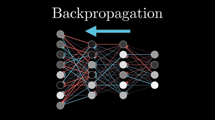
Backpropagation is workhorse behind training neural networks and understanding what’s happening inside this algorithm is atmost importance for efficient learning. This post gives in depth explanation of Backpropagation for training neural networks.

Below are the contents:

1. Notation to represent neural network
2. Forward propagation
3. Contribution of error from a single neuron
4. Main equations of Backpropagation
5. Chain rule of Calculus
6. Proof of 4 equations of Back Propagation
7. Entire Process of Backpropagation and Gradient descent

1. Notation to represent a neural network:

I will be using a 2 layer neural network as shown below through out this post as our running example.

• w_jk^[l] - Weight for connection from k^th neuron in layer (l-1) to j^th neuron in layer l
• b_j^[l] - Bias of j^th neuron in layer l
• a_j^[l] - Activation of j^th neuron in layer l

2) Forward propagation:

Below is the calculation that happens as part of forward propagation in single neuron

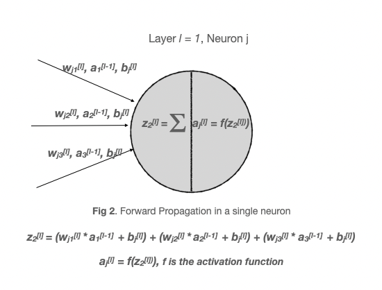
So the activation at any neuron in layer l can be written as

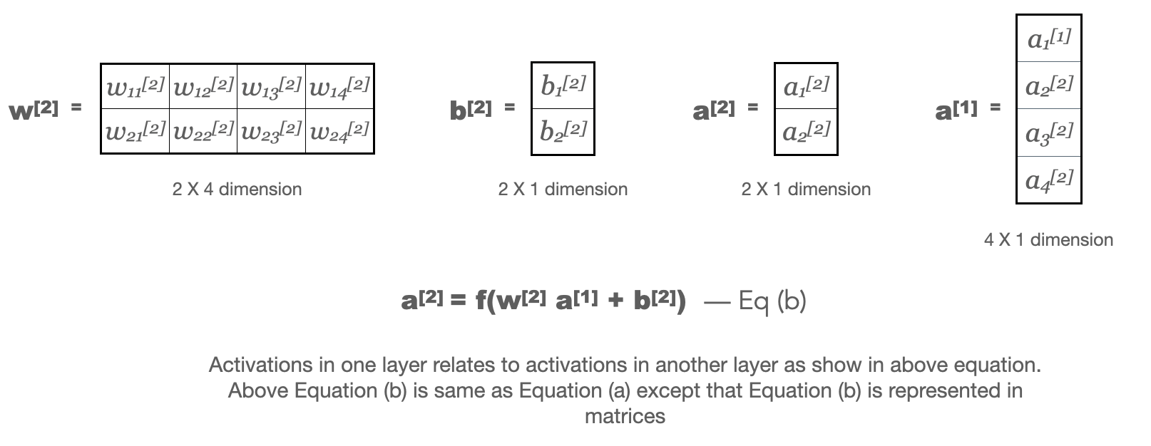
\[a_j^{[l]} = g_{\text{activ}}(\sum_{k} w_{jk}^{[l]} a_{k}^{[l-1]} + b_{j}^{[l]})\tag{a}\]

Matrix representation:

For Neural network in Fig 1 above,

w^[l] - Weight matrix for layer l

We use equation (a) from above to calulate activations for every layer but all calculations are done using matrix mulitiplcations as they are very fast

Main goal of backpropagation is to understand how varying individiual weights of network changes the errors made by the network. But how do we calculate error made by the nextwork. We use term called cost function to get estimate of error. Cost gives estimate of how bad or good our network predictions are. This is function of actual label and predicted value

\[c_x = f(y^i,yhat)\]

where is the actual label or truth of data point i and yhat is the prediction from neural network.

We usually get cost for individual training example and overall cost would be average of cost over all the training examples. Written as

\[C = \frac{1}{n} \sum_{x} c_x\]

Lets use quadratic cost for illustration in our example which is \(c_x = \frac{1}{2} (y^i - yhat)^2\). Here yhat would be exactly same as activations/output of final layer of neural network

\[c_x = \frac{1}{2} (y^i - a^{[L]})^2\]

\(a^{[L]}\) is a vector as shown in fig.3 and L = 2 for our example neural network of fig.1. Since \(y^i\) is fixed for any training example, so cost \(c_x\) is function of \(a^{[L]}\)

Back propagation is all about understanding how changing the weights and biases in a network changes the cost function \(c_x\)

Using Back propagation we calculate \(\frac{\partial c_x }{\partial w}\) and \(\frac{\partial c_x }{\partial b}\) for single training example and then from this we can calculate \(\frac{\partial C }{\partial w}\) and \(\frac{\partial C }{\partial b}\) by overaging over training examples. If we see per node, then our goal is to find \(\frac{\partial C }{\partial w_{jk}^{[l]}}\) and \(\frac{\partial C }{\partial b_{j}^{[l]}}\) for any layer l .

3) Contribution of error from a single neuron

Lets say we change our parameters and biases coming in to a neuron j of layer l. We know forward propagation equation as below. k represents all the k nodes of previous layer l-1

\[z_j^{[l]} = \sum_{k} w_{jk}^{[l]} a_{k}^{[l-1]} + b_{j}^{[l]}\]

So as we change parameters \(w_{jk}^{[l]}\) and \(b_{j}^{[l]}\) corresponding to any neuron j of layer l then output \(z_j^{[l]}\) generated in that neuron also changes and this in turn finally change our cost function \(c_x\). We can write this change as \(\frac{\partial c_x }{\partial z_{j}^{[l]}}\). So we can define contribution of change/error from this single neuron as

\[e_j^{[l]} = \frac{\partial c_x }{\partial z_{j}^{[l]}}\]

Using Backpropagation we can compute \(e_j^{[l]}\) first and then derive \(\frac{\partial c_x }{\partial w_{jk}^{[l]}}\) and \(\frac{\partial c_x }{\partial b_{j}^{[l]}}\) from this error.

4) Main equations of Backpropagation

Equation 1 - Equation for error in output layer \(e_j^{[L]}\)

\[\color{green}{e_j^{[L]} = \frac{\partial c_x }{\partial a_{j}^{[L]}} g'_{\text{activ}}(z_{j}^{[l]})}\tag{1}\]

For our example cost function \(c_x = \frac{1}{2} (y^i - a^{[L]})^2\),

\[\frac{\partial c_x }{\partial a_{j}^{[l]}} = \frac{1}{2} * 2 * (y_j - a_{j}^{[l]}) * (-1) = (a_{j}^{[l]} - y_j)\]

Equation 2 - Error of a layer in terms of error of next layer

\[\color{green}{e_j^{[l]} = \sum_{k} w_{kj}^{[l+1]} e_{k}^{[l+1]} g'_{\text{activ}}(z_{j}^{[l]})}\tag{2}\]

So once we know error in latter layers, this equation implies we can calculate error in initial layers. So by using equation 1 and equation 2, we can compute error \(e_j^{[l]}\) for any layer in the network.

Equation 3 - Rate of change of cost with respect to bias

\[\color{green}{\frac{\partial c_x }{\partial b_{j}^{[l]}} = e_j^{[l]}}\tag{3}\]

Equation 4 - Rate of change of cost with respect to NN weights

\[\color{green}{\frac{\partial c_x }{\partial w_{jk}^{[l]}} = a_{jk}^{[l-1]} e_j^{[l]}}\tag{4}\]

Now lets try to prove the above 4 equations and get some intuition of what we are getting from them. But before that lets understand chain rule of calculus which we help us going forward

5) Chain rule of Calculus

Lets say we have 3 variables and they are related as shown below

\[\frac{\partial c }{\partial z} = \frac{\partial c }{\partial a} * \frac{\partial a }{\partial z}\]

6) Proof of 4 equations of Back Propagation

Proof of equation 1

We have shown above that error from single neuron as \(e_j^{[l]} = \frac{\partial c_x }{\partial z_{j}^{[l]}}\)

Lets see again the simple calculations happening inside one single neuron of last layer L

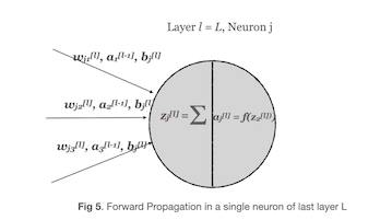
So, in equation form we can write as

\[z_j^{[L]} = \sum_{k} w_{jk}^{[L]} a_{k}^{[L-1]} + b_{j}^{[L]}\] \[a_j^{[L]} = g_{\text{activ}}(z_{j}^{[L]})\]

Now we can apply chain rule to above chain of equations and substituting \(a_j^{[L]}\) for \(g_{\text{activ}}(z_{j}^{[L]})\)

\[\begin{align} \color{blue}{e_j^{[L]}} &= \frac{\partial c_x }{\partial z_{j}^{[L]}} \\ &= \frac{\partial c_x }{\partial a_{j}^{[L]}} \frac{\partial a_{j}^{[L]} }{\partial z_{j}^{[L]}} \\ &= \frac{\partial c_x }{\partial a_{j}^{[L]}} \frac{\partial g_{\text{activ}}(z_{j}^{[L]})}{\partial z_{j}^{[L]}} \\ &= \color{blue}{\frac{\partial c_x }{\partial a_{j}^{[L]}} g'_{\text{activ}}(z_{j}^{[l]})} \end{align}\]

This is exact equation 1

Proof of equation 2

We know the error from single neuron as \(e_j^{[l]} = \frac{\partial c_x }{\partial z_{j}^{[l]}}\)

Lets use example 2 layers of a neural network to understand how we can use chain rule here

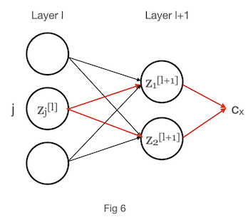
Using above fig 6 and chain rule we can write error in neuron j of layer l as

\[\begin{align} {e_j^{[l]}} &= \frac{\partial c_x }{\partial z_{j}^{[l]}} \\ &= (\frac{\partial c_x }{\partial z_{1}^{[l+1]}} \frac{\partial z_{1}^{[l+1]} }{\partial z_{j}^{[l]}}) + (\frac{\partial c_x }{\partial z_{2}^{[l+1]}} \frac{\partial z_{2}^{[l+1]} }{\partial z_{j}^{[l]}}) \\ &= \sum_{k=2} \frac{\partial c_x }{\partial z_{k}^{[l+1]}} \frac{\partial z_{k}^{[l+1]} }{\partial z_{j}^{[l]}} \end{align}\]

we can extrapolate this for any value k and replacing \({e_k^{[l+1]}}\) for \(\frac{\partial c_x }{\partial z_{k}^{[l+1]}}\) gives

\[\begin{align} {e_j^{[l]}} &= \sum_{k} \frac{\partial z_{k}^{[l+1]} }{\partial z_{j}^{[l]}} {e_k^{[l+1]}}\tag{5} \end{align}\]

From forward propagation, we know

\[\begin{align} {z_k^{[l+1]}} &= \sum_{j} w_{kj}^{[l+1]} a_{j}^{[l]} + b_{k}^{[l+1]} \\ &= \sum_{j} w_{kj}^{[l+1]} g_{\text{activ}}(z_{j}^{[L]}) + b_{k}^{[l+1]}\tag{6} \end{align}\]

where j are number of nodes in layer l and k are number of nodes in layer l+1. Taking partial derivate of equation 6 with \(z_j^{[l]}\) gives

\[\frac{\partial z_k^{[l+1]}}{\partial z_j^{[l]}} = w_{kj}^{[l+1]} g'_{\text{activ}}(z_{j}^{[l]})\]

Now we can substitute above \(\frac{\partial z_k^{[l+1]}}{\partial z_j^{[l]}}\) in to equation 5 gives

\[\begin{align} \color{blue}{e_j^{[l]}} &= \color{blue}{\sum_{k}} \color{blue}{w_{kj}^{[l+1]}} \color{blue}{g'_{\text{activ}}(z_{j}^{[l]})} \color{blue}{e_k^{[l+1]}} \end{align}\]

which is exact equation 2

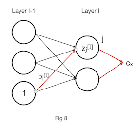
Proof of equation 4

Consider below picture for understanding of proof

Again following chain rule,

\[\begin{align} \frac{\partial c_x}{\partial w_{jk}^{[l]}}&= \frac{\partial c_x }{\partial z_{j}^{[l]}} \frac{\partial z_{j}^{[l]} }{\partial w_{jk}^{[l]}}\tag{7} \end{align}\]

We also know that from forward propagation,

\[z_j^{[l]} = \sum_{k} w_{jk}^{[l]} a_{k}^{[l-1]} + b_{j}^{[l]}\]

Taking derivative of above equation with \({w_{jk}^{[l]}}\) gives \(a_k^{[l-1]}\) and we can substitute this in equation 7. Also from definitin of error \(\frac{\partial c_x }{\partial z_{j}^{[l]}}\) = \(e_j^{[l]}\). Substituting in equation 7 gives

\[\begin{align} \color{blue}{\frac{\partial c_x}{\partial w_{jk}^{[l]}}} &= \color{blue}{e_j^{[l]} a_k^{[l-1]}} \end{align}\]

which is exact equation 4

Proof of equation 3

Consider below picture for understanding of proof

Again following chain rule,

\[\begin{align} \frac{\partial c_x}{\partial b_{j}^{[l]}}&= \frac{\partial c_x }{\partial z_{j}^{[l]}} \frac{\partial z_{j}^{[l]} }{\partial b_{j}^{[l]}}\tag{8} \end{align}\]

We know that from forward propagation,

\[z_j^{[l]} = \sum_{k} w_{jk}^{[l]} a_{k}^{[l-1]} + b_{j}^{[l]}\]

Taking derivative of above equation with \({b_{j}^{[l]}}\) gives 1 and we can substitute this in equation 8. Also from definitin of error \(\frac{\partial c_x }{\partial z_{j}^{[l]}}\) = \(e_j^{[l]}\). Substituting in equation 8 gives

\[\begin{align} \color{blue}{\frac{\partial c_x}{\partial b_{j}^{[l]}}} &= \color{blue}{e_j^{[l]}} \end{align}\]

which is exact equation 3

Using equations 1 and 2, we get contribution of errors for every layer and node of neural network. Using these and equations 3 and 4 we can compute rate of change of cost with respect to parameters W and b.

7) Entire Process of Backpropagation and Gradient descent

References:

1) Micheal A. Nielsen, “Neural Networks and Deep Learning”

2) Deep learning Nanodegree from Udacity

3) Deep learning specialization by Andrew Ng