This article talks about the Reformer architecture in NLP which solves the memory efficiency challenges faced by Transformers architecture for long sequences.

Knowledge about transformer architecture is necessary to understand this article. For those who are new to transformer architecture have a look at Transformers

Transformer Complexity:

Recent trend in Natural Language Processing is to use Transformer Architecture for a wide range of NLP tasks including but just not limited to Machine translation, Question-Answering, Named entity recognition, Text Summarization. It takes advantage of parallelization and relies on attention mechanism to draw global dependencies between input and output. It was shown to successfully outperform LSTM’s and GRU’s on wide range of tasks.

In my recent blog Transformers I tried explaining Transformer architecture for machine translation. For more detail on the complete transformer operation, have a look at it.

Transformer models are also used on increasingly long sequences. Up to 11 thousand tokens of text in a single example were processed in (Liu et al., 2018) but the problem is transformers performed well on short sequences but it will easily run out of memory when run on long sequences. Let’s understand why

• Attention on sequence of length L takes L² time and memory. For example, if we are doing self-attention on two sentences of length L then we need to compare each word in the first sentence with each word in the second sentence which is L X L comparison = L². This is just for one layer of the transformer.

• We also need to store activations from each layer of forward so that they can be used during the backpropagation

This is not a problem for shorter sequence lengths but take an example given in the Reformer paper. 0.5B parameters per layer = 2GB of memory, Activations for 64k tokens(long sequence) with embed_size = 1024 and batch_size = 8 requires another 2GB of memory per layer. If we have only one layer we can easily fit entire computations in memory. But recent transformer models have more than one layer(GPT3 has 96 layers). So total memory requirement would be around 96 * 4GB ~ 400 GB which is impossible to fit on a single GPU. So what can we do to efficiently run transformer architecture on long sequences. Here comes Reformer.

Overview of Reformer:

Reformer solves the memory constraints of transformer model by adding

• Locality sensitive hashing attention

• Reversible residual networks

• Chunked feed forward layers

Let’s understand each component in detail.

Locality sensitive hashing attention(LSH attention):

Before we start LSH attention, lets discuss briefly how standard attention works in transformers. For detailed information have a look at my article on transformers.

We have query, key, and value vectors generated from input embedding vectors. We match each query with every key to find the similarity that query is a match for key i.e, every position needs to look at every other position. So if the sequence is of length L then we need to compute L² comparisons using the dot product. These are called attention scores. Softmax is then applied to the result to obtain the weights on the values. Now value vector is multiplied to get a new representation of the input.

Entire calculation can be seen as

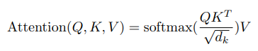
The self-attention dot product grows as the size of the input squared. For example, if one wished to have an input size of 1024, that would result in 1024² or over a million dot products for each head. This is one of the bottlenecks in current transformer architecture for long sequences. Reformer solves this problem by an approach called Locality Sensitive Hashing(LSH) attention.

The transformer uses 3 different linear layers(with different parameters) on the input to generate Q, K, V. But for LSH attention, queries and keys(Q and K) are identical. Authors called the model that behaves like this as shared-QK Transformer.

Intution behind LSH attention

For any query q_i ∈ Q = [q₁,q₂,….,q_n], do we really need to compute comparision or dot product with each and every key k_i ∈ K = [k₁,k₂,….,k_n]. If we want to approximate standard attention on long sequences the answer is NO. Lets understand intuition behind LSH with simple example below. Image is from Google Blog

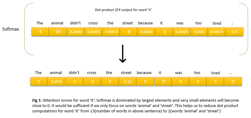
Above is a snapshot of attention weights when the transformer is trying to re-represent the word it. In the left figure above, the word animal is receiving a higher score followed by the word street. This is perfect as the sentence ends with tired and what is tired refers to animal. In the right figure above, the sentence ends with the word wide and on the same lines transformer also gave a high score to the word street and then followed by the word animal. Until now this is just standard attention going on. But if we see the above two pictures, only a few words are receiving scores in both cases and words like didn’t, cross, the, because, was, too have scores close to 0. Idea is that we apply softmax after the dot product and softmax is dominated by the largest elements. For each query q_i (in above example this is word it), we only need to focus on the keys in K that have higher similarity scores with q_i i.e., that are closest to q_i (in above example these are words animal, street)

Understanding the above example with dummy values

So for any query q_i ∈ Q = [q₁,q₂,….,q_n] we need to find all the keys k_i ∈ K = [k₁,k₂,….,k_n] that have larger dot product i.e., nearest neighbours among keys. But how can we find these? Answer is Locality sensitive hashing

But as mentioned above in LSH attention Q and K are identical. So it would suffice if we can find query vectors that are closest to each query vector q_i. What Locality sensitive hashing does is it clusters query vectors into buckets, such that all query vectors that belong to the same bucket have high similarity(so higher dot product and higher softmax output). And LSH attention approximates attention by taking the dot product between queries that are in the same bucket. This greatly reduces computation as now for a given query vector q_i we just compute dot product with subset of all other query vectors in [q₁,q₂,….,q_n].

Let’s understand this with a simple example.

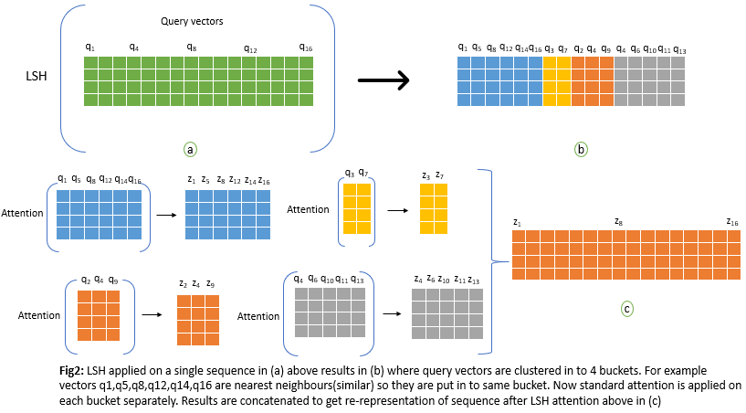
In above figure n_q = 4. The above logic works fine but there is one inefficiency in the way we calculate LSH attention, which is attention function operates on different sizes of matrices above, which is suboptimal for efficient batching in GPU or TPU. To remedy this authors of the paper used a batching approach where chunks of m consecutive queries attend to each other. But this might split a single bucket into more than one chunk. So to take care of this, a chunk of m consecutive queries will also attend one chunk back as shown below. This way, we can be assured that all vectors in a bucket attend to each other with a high probability.

With hashing, there is always a small probability that similar items may fall in different buckets. This probability can be reduced by doing multiple rounds of hashing with nrounds = n_h in parallel. For each output position(word) i, multiple vectors(z_i¹,z_i²,z_i³,…z_i^n_h) are computed and finally combined in to one.

We have to keep in mind that all the above calculations are just for one head of attention. Similar calculations will be performed in parallel for n_heads as in multi-headed attention of transformers and combined. For a detailed explanation of multi-headed attention have a look at my blog on transformers.

As a side note, in a standard transformer, a query(q_i) is allowed to attend to itself. But in the reformer, this is not allowed as the dot product of query q_i with itself will almost always be greater than the dot product of a query vector with a vector at another position.

LSH attention replaces the O(L²) factor in attention layers with O(LlogL) and so allows operating on long sequences but we have one more problem caused by the requirement to store activations in all layers for backprop.

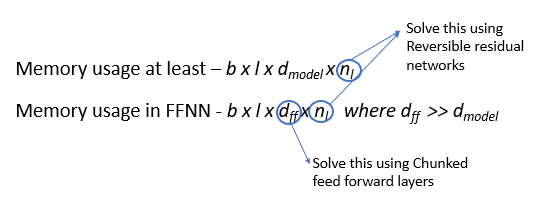
Memory use of the whole model for storing activations with n_l layers is at least b.l.d_model.n_l. Even worse: inside the feed-forward layers of Transformer this goes up to b.l.d_ff.n_l where d_ff » d_model. Here b = batch size, l = length of sequence, d_model = Embedding dimension and d_ff = Size of FFNN

Reversible residual networks

The transformer network proceeds by repeatedly adding activations to a layer in the forward pass i.e., network store activations from each layer of forward pass so that they can be used during backpropagation. Activations for each layer are of a size b.l.d_model, so the memory use of the whole model with n_l layers is at least b.l.d_model.n_l. If we are processing longer sequences with a lot of layers in the architecture then we cannot fit all these activations in a single GPU. This is the fundamental efficiency challenge. Let’s understand this with the example below.

From the above figure, for example, during a backward pass to calculate the gradient of S we need to have access to output Z, input X, and gradient of Z. So values of Z and X have to be saved somewhere to successfully perform backward propagation. The same problem would occur with calculating other gradients too. So we need to store activations like these for each and every layer and as the length of the input sequence increases then we cannot fit all these activations on a single GPU.

Do we really need to store all these intermediate activations in memory for a backward pass? Can we recalculate these activations on the fly during the backward pass? If we can do this we could save a lot of memory and the fundamental challenge would be solved. Authors of the reformer paper solved the problem by using Reversible residual networks in the architecture. The main idea is to allow the activations at any given layer to be recovered from the activations at the following layer, using only the model parameters. Let’s understand these in detail with just one layer but logic would be the same even for multiple layers.

The key idea is that we start with 2 copies of inputs, then at each layer, we only update one of them. The activations we do not update will be the ones used to compute the residuals. With this configuration, we can now run the network in reverse. Let’s understand how this new architecture solves our memory problem.

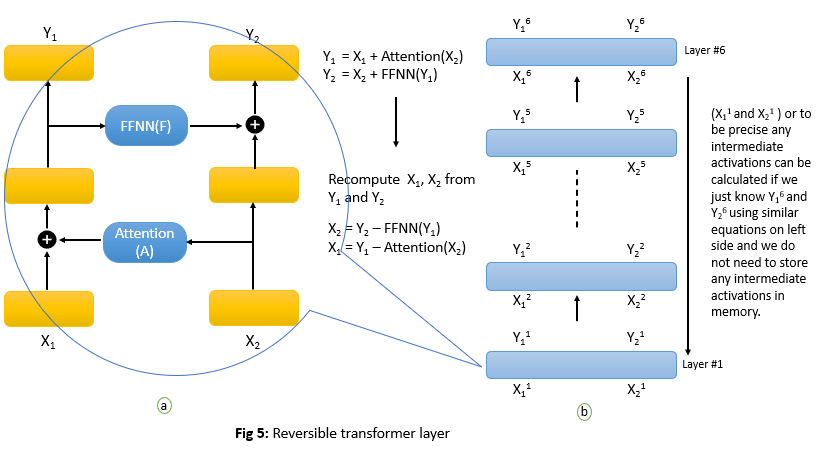
Layer Normalization is moved inside the residual blocks in above figure. So if we have outputs Y₁ and Y₂ then we can easily recalculate X₁ and X₂ during backpropagation using equations in above figure with out having to store X₁ and X₂ in memory((a) above). Just assume if Y₁ and Y₂ are generated outputs after 6^th layer in reformer and stored in memory then we can recalculate on fly all the intermediate outputs from all the layers with out having to store them in memory((b) above)

Since the reversible Transformer does not need to store activations in each layer we get rid of the n_l term in b.l.d_model.n_l we have seen above. So the memory use of the whole model with n_l layers is b.l.d_model.

Chunked feed forward layers

But we still have the problem of larger dimensions in feed forward layers d_ff. Usually, this dimension is set to 4K. To give a background, in transformers architecture attention layer is followed by 2 feed forward layers. From figure 4 matrix Z^’ is input to FFNN. The entire forward pass through FFNN is shown below.

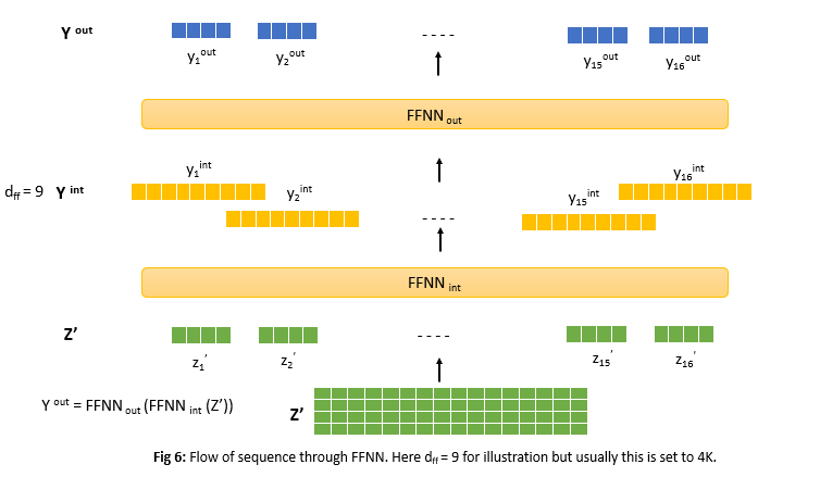
It is important to understand that feed forward layers process sequences independent of tokens and in parallel which means output y₁^out depends only on z₁^’, y₂^out depends only on z₂^’ and so on.

From above figure we can see output dimensions of FFNN_int is d_ff = 9 for illustration but usually its set to large number(4000) and output of FFNN_out is d_model = 4(usually this dimension is same as input to FFNN). Authors observed that d_ff usually tends to be much larger than d_model. This means that tensor Y_int of dimension d_ff X n allocates a significant amount of the total memory and can even become the memory bottleneck. Do we really need to compute and save Y_int when Y_out is what we need? We somehow need to overcome this problem and the answer is Chunked feed forward layers

Intutition

Instead of processing the entire sequence through FFNN to generate Y_int and then Y_out we only process one chunk at a time through 2 layers of FFNN and finally, all chunks are concatenated to generate Y_out. This method solves memory problem but takes a longer time to process.Let’s understand this with an example.

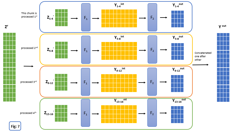
In above fig, input is processed with chunks of size 4. So instead of storing entire Y^int of size l X d_ff (l = 16 above) in memory during forward pass, now with chunked feed forward layers we store just tensor of size 4 X d_ff (in general chunk_size X d_ff) in memory at a time and finally results are concatenated.

Conclusion

Reformer takes the soul of the transformer and each part of it is re-engineered very efficiently using LSH attention, Reversible residual networks, and Chunked feed forward layers so that it can be executed efficiently on long sequences even for models with a large number of layers.

References:

1) Reformer: The Efficient Transformer(Nikita Kitaev et al., 2020)

2) Natural language processing specialization - Coursera

3) Google AI blog on Reformer

4) The Reformer - Pushing the limits of language modeling by HuggingFace