Attention is all you need - The Transformer

This article talks about the famous Transformers architecture in Natural Language Processing.

Background:

Historically RNN’s like LSTM’s and GRU’s are widely used architectures for most natural language understanding tasks like Machine translation, language modeling. They performed decently well but one major drawback is RNN’s process data sequentially. This inhibits parallelization, so the more words we have in the input sequence, the more time it will take to process that sentence. In addition to the sequential nature of RNN’s, they suffer from vanishing gradient problems for long sequences. Transformer was introduced in paper Attention Is All You Need and it was shown that this new architecture is able to tackle the problems faced by RNN’s

I will try to explain each and every detail of Transformers in this blog post. Contents are as follows

What is Transformer?
Overview of Architecture
Encoder

1) Positional encoding

2) Self-Attention

3) Self-Attention calculation

4) Multi-head Attention

5) Feed forward Neural network layer

6) Residual connections and LayerNorm
Decoder

1) Inputs and Outputs in the decoder

2) Causal self-attention

3) Encoder-decoder attention
Final linear layer and softmax

What is Transformer?

The Transformer is an architecture whose main goal is to solve sequence-to-sequence tasks while handling long-range dependencies with ease. It totally can take advantage of parallelization and relies on attention mechanism to draw global dependencies between input and output.

In Attention Is All You Need paper, the transformer was used mainly for machine translation. So let’s keep our discussion in that domain when going through different components. Let’s say for example our goal is to translate an English sentence into a french sentence.

Overview of Architecture:

Transformer contains two main components.

Encoder
Decoder

Input to Encoder would be the English sentence and decoder outputs corresponding french sentence. Below is a simple diagram showing how a transformer is structured

Looking at the above picture, one might say that this looks exactly like sequence to sequence machine translation using RNN’s where the encoder takes input and the decoder produces output. But all the magic happens inside the big boxes above(encoder/decoder) where instead of sequential processing we have parallel processing and rely on 3 types of attention. So let’s have a look at each component in detail.

Encoder:

Encoder block is a stack consisting of 6 identical layers. Each layer has 2 sublayers. The first is a multi-head self-attention mechanism and the second is a simple position-wise fully connected feed-forward network. Let discuss with a simple picture

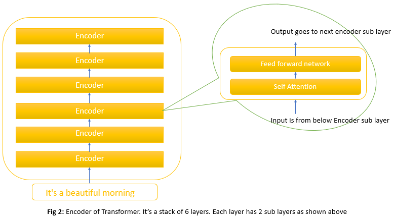
As seen above, the encoder’s input first flows through a self-attention layer that helps the encoder look at other words in the input sentence as it encodes a specific word. The outputs of the self-attention layer are fed to the feed-forward neural network. It is applied independently to each position.

The main property of the transformer is that each word in input flows through its own path in the encoder and in self-attention these input words interact and have dependencies between them. Feed forward layer does not have these interactions and since each word flows in its own path, the entire sequence can be executed in parallel as shown below.

Let’s understand all the operations that happen in the encoder with the help of 3 examples

1) They go to gym everyday

2) He is studying in third grade

3) Red cat sitting on the table

As with any NLP task, we first tokenize the sentence and convert it to numbers. After that, we convert each number(corresponding to a word) in a sentence into word embeddings. First will see how one sentence flows through an encoder using vectors and slowly will transition into using matrices for a batch of sentences

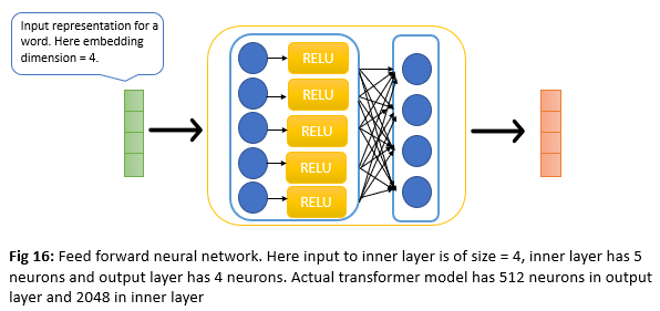
Above I used an embedding size of 4 for illustration. But in the paper, they used an embedding size of 512. So input will be a list of vectors each of size 512. First input passes through Self Attention layer and then through Feedforward neural network layer

Positional encoding

Our transformer model does not care about the actual ordering of words(all words are processed in parallel and they see all other words during attention). But for our model to make use of the order of sequence, we must add some information about the relative or absolute position of the tokens in the sequence. In other words, to give the model a sense of the order of words, we add Positional encoding to the embedding vectors. This is done both on the encoder and decoder side.

The positional encodings have the same dimension as the embeddings so that the two can be summed. The formula for calculating positional encoding is given in section 3.5 of the Attention Is All You Need paper.

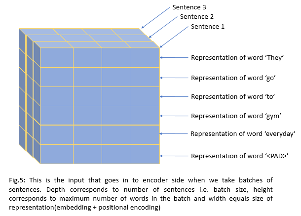
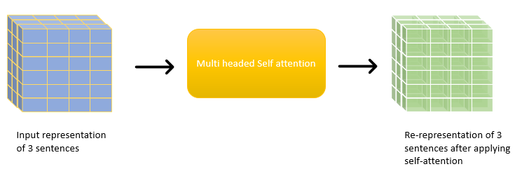
Now we know how one sentence passes through an encoder, let’s see how a batch of sentences flows. This is very important because in the real world we never deal with one sentence. Below is a simple picture that illustrates this. Again I used toy embedding of size 4 for illustration.

Above, input representation flows through the self-attention layer in the encoder. This is the heart of transformers. So let’s dig deeper

Self-Attention

Consider the sentence I arrived at the bank after crossing the…. In this sentence depending on the word which ends the sentence, the meaning and appropriate representation of the word bank changes. For example, if the ending word is river then this word bank refers to the bank of the river and if the ending word is let’s say for example road then it refers to the financial institution. So when we are re-representing a particular word, the model needs to look at surrounding words in the input sentence for clues that can help lead to a better encoding for this word.

Self Attention is the mechanism Transformer uses to bring in the information of other relevant words to the one we are currently processing

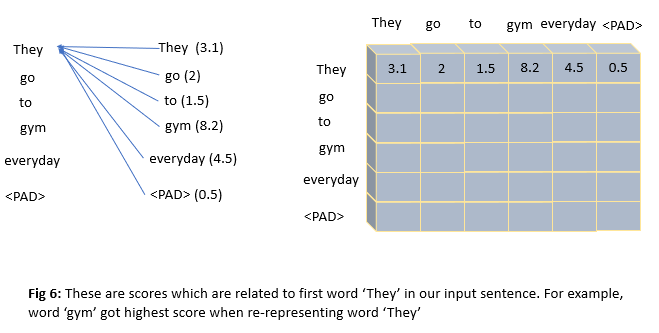
So in the above example, the word river would receive a high score i.e, when processing the word bank to compute a new representation, our model would give high attention to the word river. We can think of the final score a particular word would get is a weighted combination of representations from all surrounding words.

For each word in the input sentence, we want to get a score of all remaining words in that sentence. So somehow we need to compare each word with all others. This is the main computation involved in self-attention. We want to get something like below

Self-Attention calculation:

Let’s see now how we can calculate similarity scores as in the above fig.

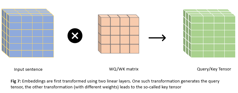
Instead of comparing embedding vectors directly, embeddings are first transformed using two linear layers. One such transformation generates query tensor(Q), the other transformation leads to key tensor(K). Since we are doing self-attention, query and key correspond to the same input sentence.

Creating Query(Q), Key(K) and Value(V) matrices

Input representation(Fig.5) is multiplied by WQ matrix(linear layer) to get Q and multiplied by WK matrix to get K. Fig.5 has dimensions of (n_seqXembed_dim) = (6X4). We will be using the WQ/WK matrix of size 4X4 for illustration. Q/K matrices will have a shape of 6X4 as shown below. For self-attention Q = K

We are projecting these input vectors into space where dot product is a good proxy for similarity. Higher the dot product score, the more similar or more attention between words.

Attention scores are calculated by the dot product between Q and K matrices i.e. Q^TK as shown below

If we see above, attention scores are large numbers. Now we apply the softmax function per row to bring all these numbers to between 0 and 1. Also good thing is that they add up to 1 for any particular word.

We have introduced Query and Key tensors so far. The last piece missing until now is the Value tensor. Value tensor is formed by a matrix multiply of the Input representation(Fig.5) with the weight matrix WV whose values were set by backpropagation. The row entries of V are then related to the corresponding input embedding.

The purpose of the dot-product is to ‘focus attention’ on some of the inputs. Dot product which is softmax(Q^TK) now has entries appropriately scaled to enhance some values and reduce others. These are now applied to the V entries.

The matrix multiply weights first column of V, representing a section of each of the input embeddings, with the first row of softmax(Q^TK), representing the similarity of word#0 and each word of the input embedding and deposits the value in Z

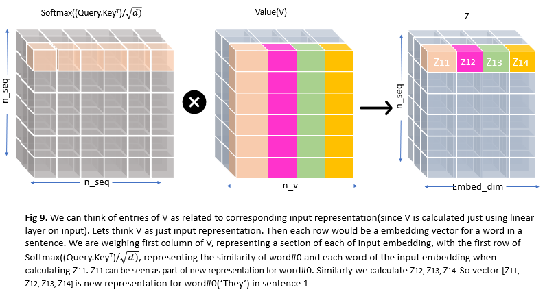
With the above calculation, we are re-representing each word in a sentence by taking into account all surrounding words’ information. This is called self-attention. It’s self because when encoding a particular sentence we are just looking at all other words in that sentence including itself but nowhere we are referring to other sentences.

Multi-head Attention:

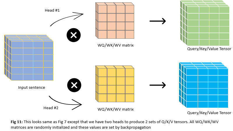
Sometimes it’s beneficial to get multiple representational subspaces for a word. For example in our sentence I arrived at the bank after crossing the river, when we calculated our representation Z, even though it uses all other words information to re-represent word bank, it could be dominated by the actual word itself. So authors of the paper thought why not use multiple attention heads(which could be applied in parallel using multiple sets of Query/Key/Value weight matrices). Let’s try to understand this with a simple example where we used 2 attention heads instead of 1 head which we were used to until now

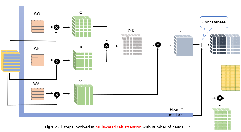
How do we calculate this? It’s very simple. Instead of using one set of Query/Key/Value weight matrices to produce one set of Q, K, V matrices, we use multiple sets of Query/Key/Value weight matrices to produce multiple sets of Q, K, V matrices. All these calculations will be done in parallel. Let’s go step by step using the number of attention heads = 2(paper used 8 attention heads)

Now we perform self-attention using 2 heads instead of 1 head as we are doing until now. As we know the first step is to calculate attention scores using dot product between Query(Q) and Key(K) vectors as shown below

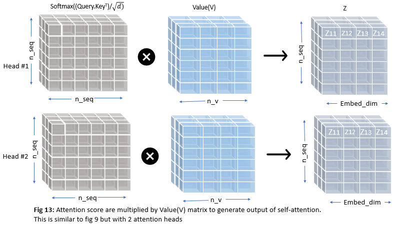
Now we have 2 sets of attention scores corresponding to 2 attention heads, we need to multiply these with Value(V) matrices as before to get the final output of self-attention

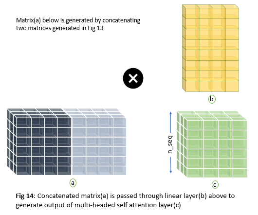
After applying multi-head attention each word in a sentence will have multiple representations(actually n_head representations where n_head is the number of attention heads). But our feed-forward layer is expecting one matrix as shown in Fig 9 but we have two matrices now in Fig 13. So we need a way to condense this information to one metric. This is done by first concatenating the two matrices and passing through the linear layer as shown below

Entire self-attention process is described below

Feed forward Neural network layer

The output of the self-attention layer will flow through FFNN as shown in Fig 4. FFNN is applied to each position separately and identically and it consists of 2 layers as shown below.

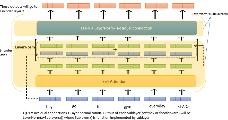
Residual connections and LayerNorm

Until now we had a look at the 2 main components of an encoder layer. Transformer architecture had 6 layers like this and the output of one layer will act as input to another layer. But there is one thing that needs to be discussed which is residual connections. We have a residual connection around each of two sub-layers in the encoder layer then followed by layer normalization. Let’s understand this with an example below. To facilitate these residual connections, all sub-layers in the model, as well as the embedding layers, produce outputs of dimension dmodel = 512. The below image uses toy dimensions of 4 for illustration

Decoder

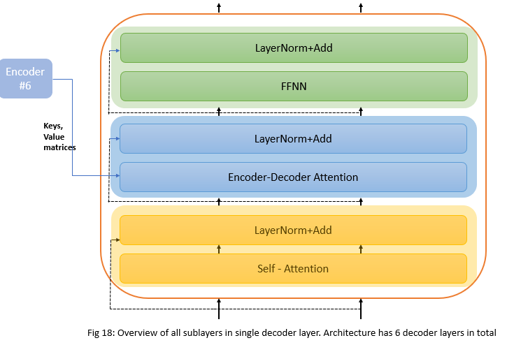
Decoder is the rightmost part of the architecture that decodes the encoder’s encoding of the input sentence. Decoder works exactly the same as encoder except that it has one more attention layer called Encoder-decoder attention. Below is an overview of decoder layers.

1) Causal self-attention - In a sentence, words only can look at previous words when generating new words. Causal attention allows words to attend to other words that are related, but an important thing to keep in mind is, they cannot attend to words in the future since these were not generated yet, they can attend to any word in the past though. This is done by masking future positions.

2) Encoder-decoder attention - For example, let’s say we are translating English to french. Input to the encoder would be English sentence and decoder outputs french sentence. Encoder-decoder attention is the one that helps the decoder focus its attention on appropriate places of the input sentence. In this layer, Queries come from the French sentence/previous decoder layer but Values and keys come from the output of the final encoder layer. This allows every position in the decoder to attend over all positions in the input sequence. This mimics the typical encoder-decoder attention mechanisms in sequence-to-sequence models.

3) Feed forward layer - FFNN is applied to each position separately and identically similar to the encoder side.

4) Residual and LayerNormalization - Similar to the encoder, the decoder also has residual connections and layer normalization.

Inputs and Outputs in decoder

Outputs in the transformer are generated token by token and the most recently generated token will be used as input for the next time step. This mimics the language modeling generation as shown below.

Causal self attention

Causal self-attention allows words to attend to other words that are already generated when generating a new word. For example in Fig 19, when generating the word belle causal self-attention allows to attend to only words C’est and une but not to word matinee since matinee is not generated yet.

Causal self-attention works the same way as self-attention of Encoder except that we need to modify calculation little to take care of the above point. This is done by masking future positions. Let’s understand this with one sentence but logic would hold true even for a batch of sentences.

Since it is just a variant of self-attention, queries and keys come from the same sentence.

English sentence: They go to gym everyday

French translation: Ils vont au gym tous les jours

Step by step:

1) Similar to self-attention we calculate Q^TK using French sentence which is matrix C in above fig. Queries(Q) and key(k) both come from the same sentence which is a French sentence here.

2) Matrix C says how similar each word in a query is to each word in key. This is called the attention weight matrix. For example, the pink strip in matrix C above says how much similar vont in query is to each word in key. So far it’s similar to self-attention. But the thing is when we are generating a word in a query, we only want to look at words that were generated until then including itself. So for example when generating the word vont, this word only wants to look at the words Ils and vont. But our similarity matrix has similarity scores even for words that come later. So we want to mask these similarity scores for words that come later.

3) This is done by adding matrix M which has all zeros on the diagonal and below and large negative numbers above the diagonal. This gives matrix f. Idea is that when we apply softmax in the next step these large negative numbers become zero as shown below.

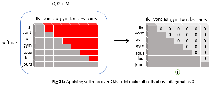
So from the matrix (a) in fig 21 above, when generating word vant it has non zero similarity values only for words Ils and vant. This helps the decoder to pay attention to only words that were generated in the past.

Steps that come after the masking were exactly the same as in the multi-headed self-attention we discussed on the encoder side.

Encoder-decoder attention

This is very similar to self-attention in encoder except that in this case Queries(Q) come from previous decoder layers, Keys(K) and values(V) come from the output of the final encoder layer. This allows every position in the decoder to attend over all positions in the input sequence.

Final linear layer and softmax

The output of the decoder will flow through the linear layer and through softmax to turn a vector of words into an actual word. These layers are applied to each individual position of the decoder separately and in parallel, as shown below

Linear layer helps to project output from decoder layers into higher dimension layer(this dimension depends on vocabulary). For example, if our french vocabulary has 20000 words then this linear layer will project our decoder output of any single token into a 20000 dimension vector. Then this 20000-dimensional vector will be passed through the softmax layer to convert into probabilities. Now we select the token with the highest probability as the output word at this token position.